

In the last few years, computer vision algorithms have been able to do many things. One amazing and dangerous thing it can do also is, generate new images, faces, voices, etc. The evolution of what these algorithms can do and if it is good is for a separate debate.
In this post, we will look at some of the fundamental techniques that power modern generative models, segmentation models, and much more. We focus on understanding about autoencoders and variational autoencoders. What makes them different? We will look at couple of real world usecases.

Finally we will build a CNN based VAE model to generate some celebrity faces. (Please do not expect an HD image)
What is Autoencoder
Autoencoders are a type of neural net architecture that contains two parts, the encoder, and the decoder. The encoder takes the input and creates a compressed form of the input. The compressed form z should contain enough information about the input that the decoder should be able to recreate the input from z.
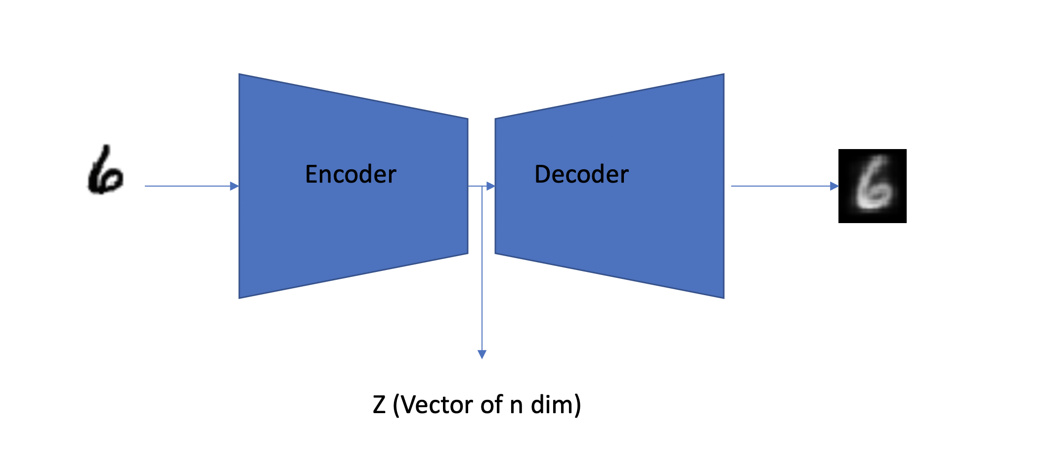
Encoder
The Encoder is similar to most of the architectures which we typically use for classification problems. For MNIST, let's use a simple network using Linear layers to reduce the dimensionality from 784 to 2.
MNIST data comes with a shape of 28,28, for simplicity we flatten it to 784
class Encode(Module):
    def __init__(self):
        self.fc1 = nn.Linear(784, 400)
        self.fc21 = nn.Linear(400, 2)

    def forward(self,x):
        x = x.view(-1,784)
        h1 = F.relu(self.fc1(x))
        return self.fc21(h1)
Decoder
Our Decoder has a tough job, it has to guess/create our input/number from just 2 numbers. To do this, the encoder has to successfully encode the most important information in z. Let's just use another simple network based out of Linear layers which would convert our z tensor back to a tensor of 784 and reshape it to 1,28,28.
We are reshaping the tensor back to image size, to match our target shape.
class Decode(Module):
    def __init__(self):
        self.fc3 = nn.Linear(2, 400)
        self.fc4 = nn.Linear(400, 784)

    def forward(self,x):
        h3 = F.relu(self.fc3(x))
        return torch.sigmoid(self.fc4(h3).view(-1,1,28,28))
Output
What is Variational Autoencoder
Variational autoencoders are very similar to auto-encoders, but they solve an important problem of helping the decoder to generate realistic-looking images from a random latent space.
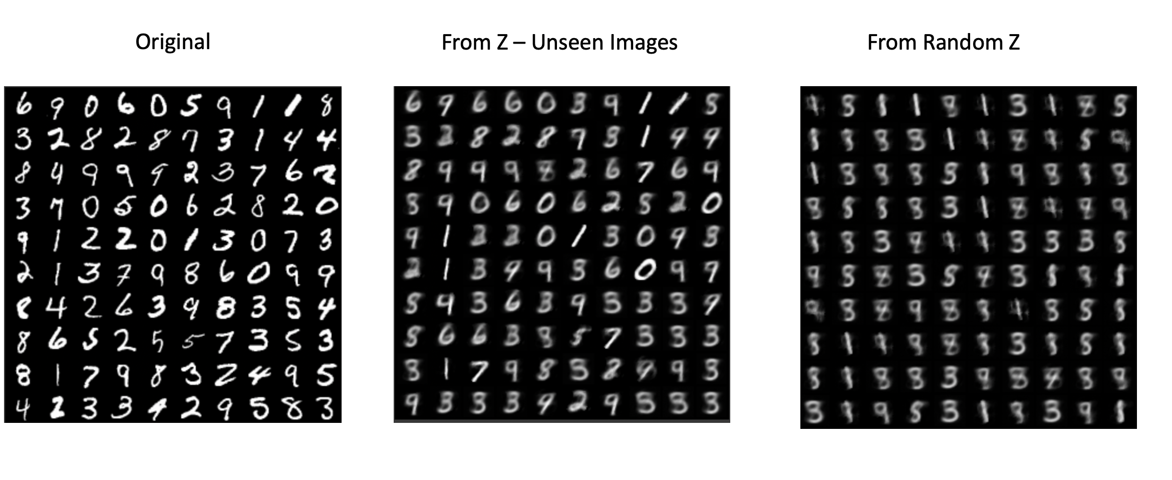
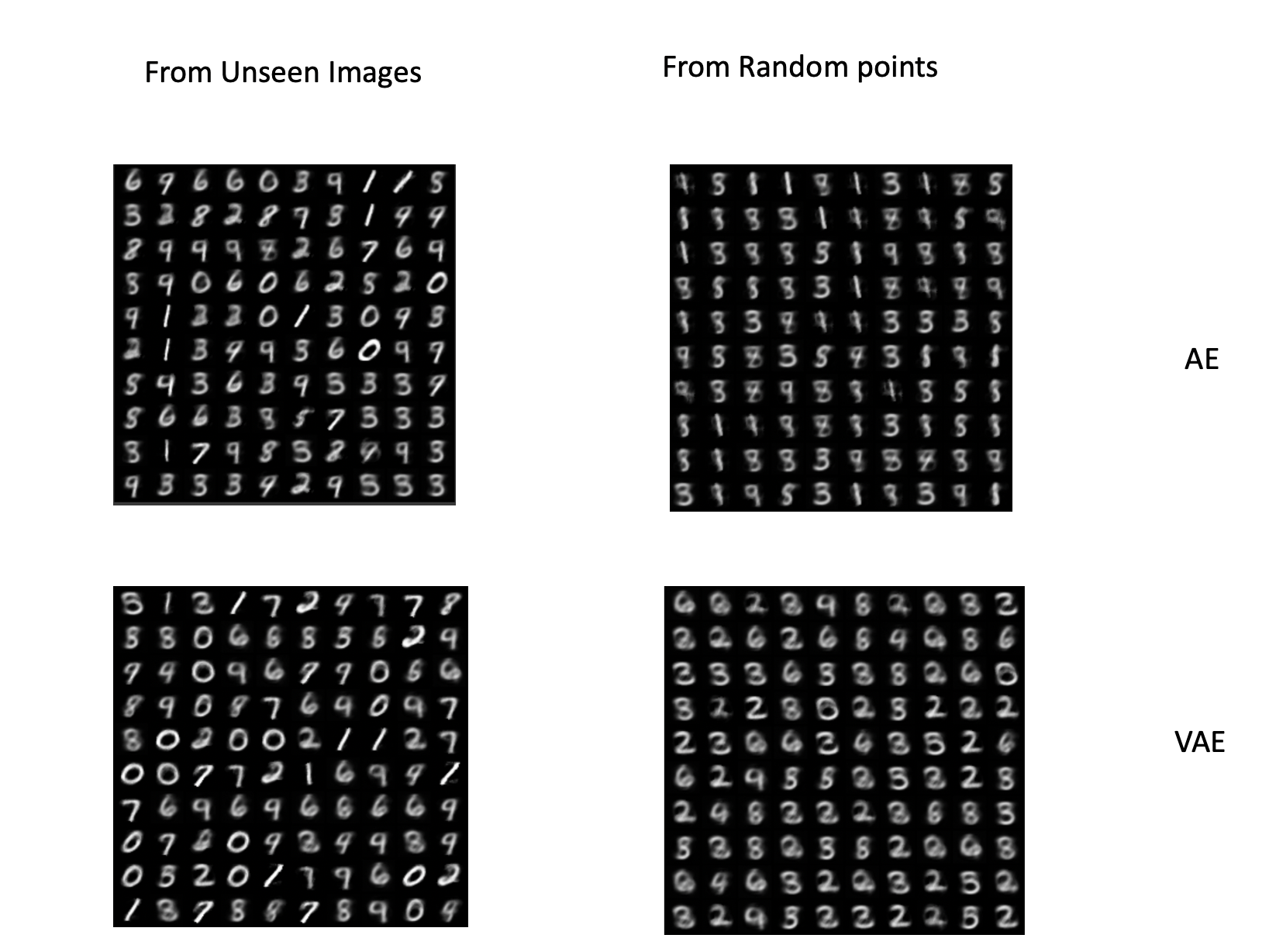
Quickly look at the output of Autoencoder and Variational Autoencoder images generated from randomly picked points. The rightmost image.
We will understand what is the difference in detail while we compare both of these techniques.
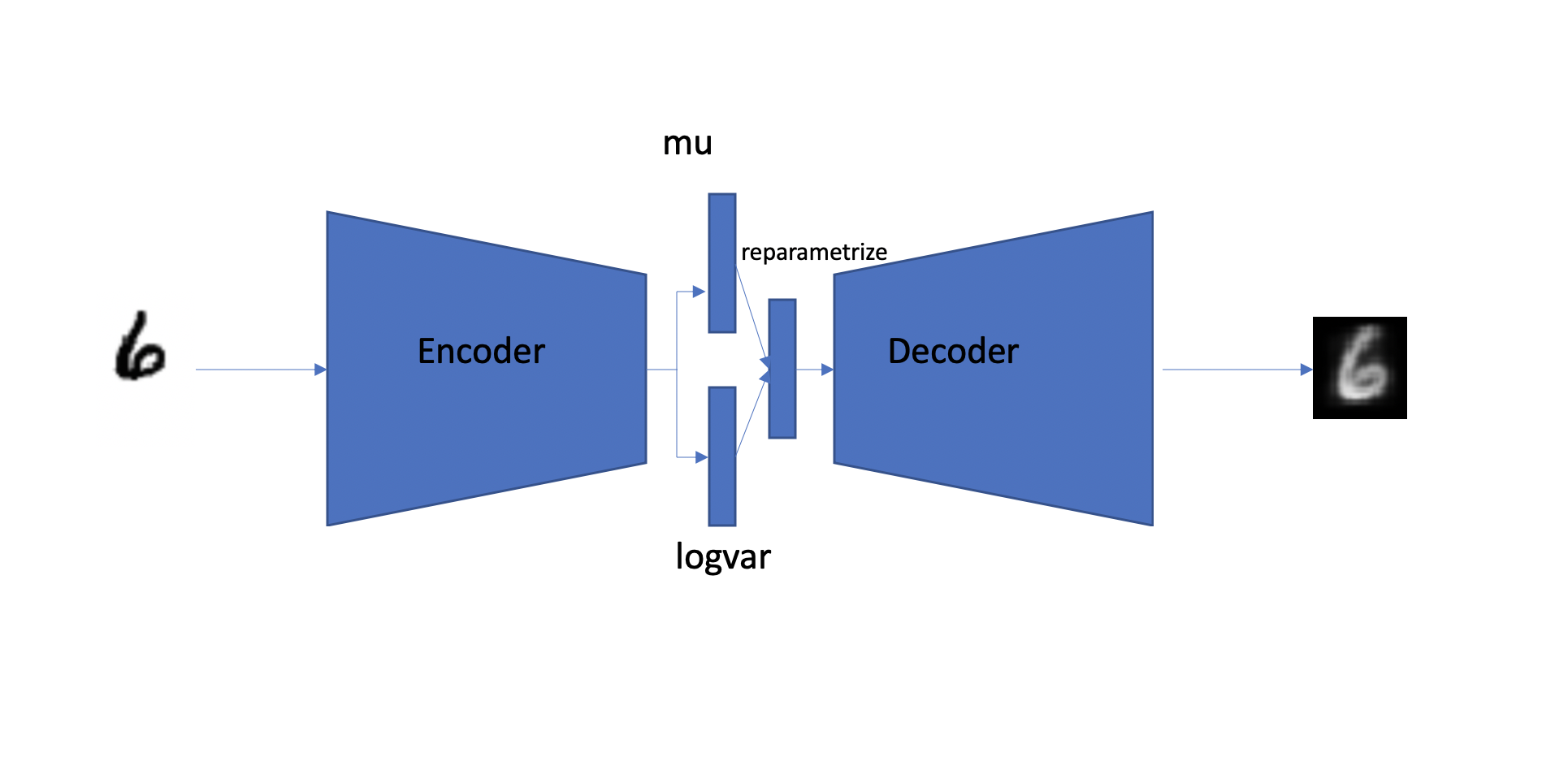
Encoder
Instead of just creating a compressed form of our input, we output 2 vectors of n dim (In our case n is 2). This would act as mean and variance for a normal distribution from which we can draw samples. If you do not come from a math background, this may sound foreign to you. Do not worry we will build the intuition required for understanding this in the next section.
class Encode(Module):
    def __init__(self):
        self.fc1 = nn.Linear(784, 400)
        self.fc21 = nn.Linear(400, 2)
        self.fc22 = nn.Linear(400, 2)

    def forward(self,x):
        x = x.view(-1,784)
        h1 = F.relu(self.fc1(x))
        return self.fc21(h1),self.fc22(h1)
Decoder
The Decoder for variational autoencoder can be the same as for autoencoder. If you are confused about why is our encoder spitting 2 tensors while our decoder only relies on only 1 then please wait till the next section, where we will be looking at the missing puzzle.
class Decode(Module):
    def __init__(self):
        self.fc3 = nn.Linear(2, 400)
        self.fc4 = nn.Linear(400, 784)

    def forward(self,x):
        h3 = F.relu(self.fc3(x))
        return torch.sigmoid(self.fc4(h3).view(-1,1,28,28))
Output
What makes them different?
We will try to understand these 2 architectures by closely looking at the outputs of each model and also by plotting the points from the latent space z. Once we understand where autoencoders suffer and how variational autoencoders succeed we will look into how variational autoencoders solve it by introducing 2 small changes.
How Autoencoders and Variational autoencoders are different?
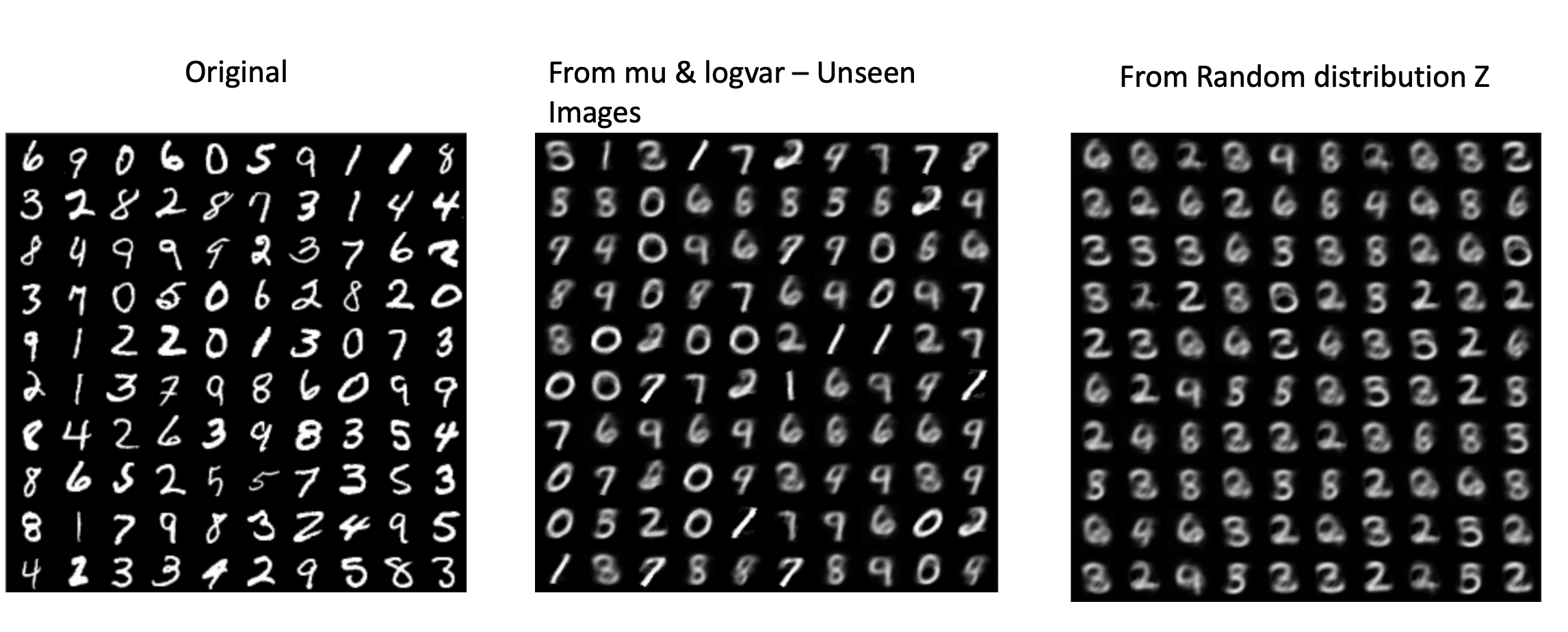
If we closely look at the images generated using AE & VAE, we can observe they have similar results. Both of the models performed well when generating images from points in the latent space which are derived from real images (The 1st column). But the results are drastically better for VAE when we pass z points drawn from random distribution (torch.randn) (images in the 2nd column).
By now it should be clear what is the problem the autoencoder is facing and what variational autoencoder is solving. But why does the autoencoder generate bad results on points drawn randomly? To understand that let's plot the output of z values of our encoder. We had the output of the last layer of the encoder, our latent space as 2 dimensions making it easier for us to plot. Let's observe what is happening here?
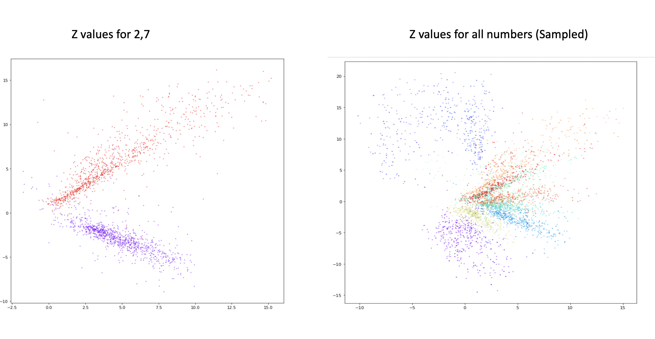
As we can observe from the above plots, our compressed data (points from latent space) is all over. From the image plotting z values for all the numbers (the right one), it is very interesting to see how our algorithm can nicely group similar numbers but there is still overlap and for some numbers, the values are spread out. Some of these points are going down till -15 and 20 to the y-axis and similarly on the x-axis. When we generate a random number using torch.randn, by default, they have a mean of 0 and a standard deviation of 1. Since the data distribution of z is all over, it makes it very difficult to generate realistic-looking images, since our autoencoder was not trained for it. We want our algorithm to learn how to group the points closer and have a distribution that is closer to normal distribution.
Let's observe how the points look for our VAE network.
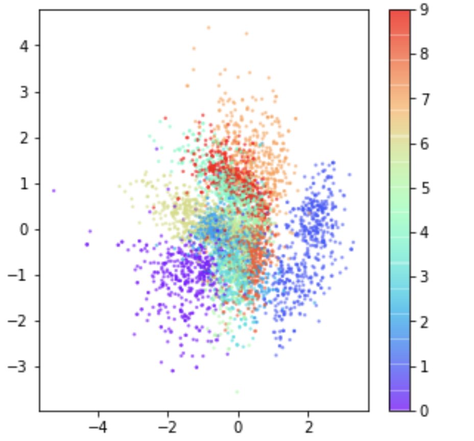
As we can observe the points from our latent space are nicely centered around 0 and points for similar classes are grouped. It is because of this distribution, the decoder in VAE was able to generate realistic-looking images when passed with points drawn from a normal distribution. VAE can achieve this by introducing 2 important changes.
Instead of creating a fixed embedding from the encoder like AE, it generates 2 tensors of n dimension, which acts as mean and standard deviation from which points can be drawn. So for a given image/input, the point in the latent space can be different in multiple passes but they will have similar mean and standard deviation.
def reparameterize(mu, logvar):
    std = torch.exp(0.5*logvar)
    eps = torch.randn_like(std)
    return mu + eps*std
Because of the nature of our sampling function
reparameterize, when even variables likemuandlogvarare constant, the function returns different values. Forcing our decoder to generate a particular category of image for any point drawn from the given distribution.
Another key change is the loss function. For an autoencoder, we can either use MSE/BCE losses, which will denote how much the model can successfully reconstruct the image. Autoencoder introduces a loss called KL divergence, which penalizes the model if the mean and standard deviation is farther from the Normal distribution that is 0 and 1. KL divergence is responsible for keeping the points from latent space around 0. The loss function for VAE combines the reconstruction loss(MSE) and KL divergence loss.
def vae_loss_function(preds,targs):
    recon_x, z,mu,logvar = preds
    recon_loss = F.mse_loss(recon_x, targs,reduction='sum')
    KLD = -0.5 * torch.sum(1 + logvar - mu.pow(2) - logvar.exp())
    return recon_loss + KLD
UseCases
Now we understand what AE and VAE are, how are they useful in real-world scenarios? Let's discuss some of their use cases.
- Compression - We can build data specific compression techniques like
zipbut only works on data types on which they are trained. During reconstruction, we lose a certain level of information. - Dimensionality reduction - We can use them like the PCA algorithm for dimensionality reduction, and use the reduced dimensionality as features for some underlying algorithms.
- Augmentation - Since our decoders can generate new images, we can use them as an augmentation technique.
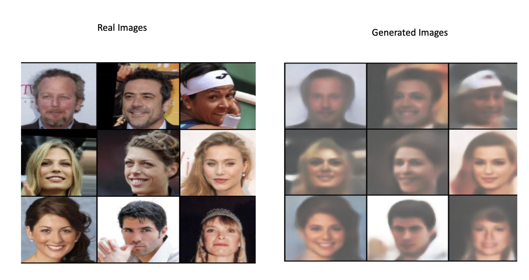
VAE for generating celebrity faces.
The MNIST dataset is always a good place to start, it helps us to focus on understanding and building our intuition. Let's try our understanding on a new dataset that contains celebrity photos.
Everything remains the same, but we will use Convolutional layers and UpSample layers for our encoder and decoder.
Encoder
We will be taking advantage of fastai ConvLayer which helps us create a custom Conv Block - Conv2d-BN-LeakyReLU. It helps us keep the code clean and consise. The input images are resized to 3,128,128 tensors and we are reducing them to 2(mu,logvar) tensors of size 500
class Encode(Module):
    def __init__(self):
        self.conv_block = nn.Sequential(ConvLayer(3,32,stride=2,act_cls=nn.LeakyReLU),
                                                       ConvLayer(32,64,stride=2,act_cls=nn.LeakyReLU),
                                                       ConvLayer(64,64,stride=2,act_cls=nn.LeakyReLU),
                                                       ConvLayer(64,64,stride=2,act_cls=nn.LeakyReLU),
                                                       Flatten()
                                       )
        self.l1 = nn.Linear(4096,500)
        self.l2 = nn.Linear(4096,500)

    def forward(self,x):
        x = self.conv_block(x)
        mu = self.l1(x)
        log_var = self.l2(x)
        return mu,log_var
For MNIST, the dimensions of
zwas only 2, we used that dimension to make it easy to plot. But for a complicated dataset, we need a much larger tensor to encode the information. We choose 500, but you can play around with the number, it acts as a hyperparameter.
Decoder
The Decoder takes a tensor of dimension 500, which is the out of reparameterize function and has to create a tensor of size 3,128,128. We can either use ConvTranspose2d or Upsample to enlarge our tensor back to the image size. We will use the UpSample layer for our decoder.
def decode_block(ni,nf,sf=2,act_cls=nn.LeakyReLU,transpose_fn=nn.UpsamplingBilinear2d):
    return nn.Sequential(transpose_fn(scale_factor=sf),ConvLayer(ni,nf,act_cls=act_cls))

class Decode(Module):
    def __init__(self):
        self.conv_block = nn.Sequential(decode_block(64,64,transpose_fn=nn.UpsamplingNearest2d),
                                        decode_block(64,64,transpose_fn=nn.UpsamplingNearest2d),
                                        decode_block(64,32,transpose_fn=nn.UpsamplingNearest2d),
                                        decode_block(32,3,transpose_fn=nn.UpsamplingNearest2d)

                                       )
        self.l1 = nn.Linear(lf,4096)

    def forward(self,x):
        x = self.l1(x)
        x = x.view(-1,64,8,8)
        x = self.conv_block(x)
        return torch.sigmoid(x)
Output from Random points
Let's look at how our complete model performs when z comes from a random normal distribution.
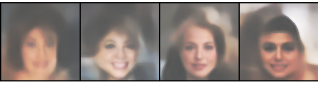
Wow, we can see faces there. Not bad for our simple model, but in 2020 we can do a lot better by trying other different techniques from the world of GAN's. In one of the future blogs, let's look at some of the techniques that we can use to generate more realistic looking images.
Missing pieces
Some of the pieces we did not cover are creating the data pipeline, training the model, and analyzing the results. We used fastai for building data pipeline and training. The below code shows how we built a data pipeline using a fastai datablock API and how we trained.
# Data pipeline
db = DataBlock(blocks=(ImageBlock(),ImageBlock()),
               get_items=get_image_files,
               item_tfms=[Resize(128)],
               splitter=RandomSplitter(0.05))
dls_c = db.dataloaders(source=celeb_path/'img_align_celeba',bs=64)

#Training VAE model

learn = Learner(dls_c,CelebVAE(),loss_func=celeb_loss_function,opt_func=Adam)
learn.fit_one_cycle(50,lr=1e-3)
If you are new to datablock API, I would recommend checking out one of our previous blog in which we went in detail about building a datablock. For analyzing the results we used the famous matplotlib and it is self-explanatory.
If you want to quickly try out this project or use this technique in your cool project then check out JarvisCloud - A simple and affordable GPU cloud platform.
Conclusion
We learned how to build autoencoders and variational autoencoders. We learned how variational autoencoders can be trained to generate inputs like images and audio from points drawn from a random distribution. Several other new techniques are developed and these concepts act as fundamentals for their understanding. We will explore more about such techniques in the future.