

Transfer learning has become a key component of modern deep learning, both in the fields of CV and NLP. In this post, we will look at how to apply transfer learning for a Computer Vision classification problem. Along the way I will be showing you how to tweak your neural network to achieve better results. We are using PyTorch for this, but the techniques that we learn can be applied across other frameworks too.

By the end of the blog, we would have learned 7 important tricks that we can use to improve our deep learning model results. The val_acc shows how each technique performs on the choosen validation dataset.
| Experiment Name | val_acc |
|---|---|
| As feature extractor | 0.983648 |
| Feature extractor with BN layer in eval mode | 0.987736 |
| Train just the BN layer in the pretrained network | 0.990881 |
| BN is completely trainable, with discriminative learning. | 0.993711 |
| BN is not trainable, with discriminative learning. | 0.991509 |
| AdaptiveConcatPooling | 0.990252 |
| Classifier/Head - With a deeper network | 0.992767 |
What is transfer learning?
In the world of Deep learning, training the model from scratch (Random points) has been the standard practice in the past. Let's say we are training a model from scratch to identify if a given image contains an animal or a building. It has to learn several important features like, what is eye and nose or windows and floors to successfully differentiate between an animal and a building. After training the model for several epochs the model successfully learns it. Now let's say we got another task of building a model to identify if a given image contains a dog or cat, then we generally train a new model from scratch. This has been the standard in the past.
We humans, do not do tasks like this. We use our pre-existing knowledge and learn/upskill only the new skill required to finish a task. How about using a model that is already trained to identify images in the real world for our task. The techniques that are used for using a pre-trained model for training a model to identify a completely new task is called transfer learning.
For computer vision, most of the pre-trained models are trained on a very popular dataset called Imagenet containing 1000 categories. We would be using one such model called resnet34, which is the go-to model in recent years as it is very fast and very stable during hyperparameter tuning.
Dataset
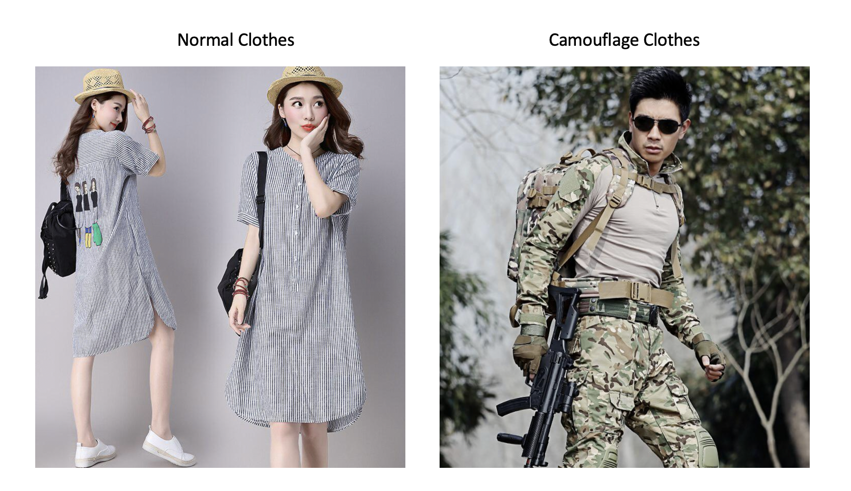
Kaggle provides a lot of datasets, let's pick one that contains images which are not part of Imagenet categories. We will take a dataset that contains images of persons wearing normal clothes vs camouflage clothes.
The images come in 2 folders. Let's create a train and validation split so that we can benchmark different techniques against the same data. For simplicity, I am just picking the first 20% of images in each folder for our validation. The below code will create our train and validation split.
#We are taking 20 percent of data
valid_pct = int(7950*0.2)

def copy_files(files,dst_path):
    for o in files:o.rename(dst_path/o.name)

for cloth_type in ['camouflage_clothes','normal_clothes']:
    files = list((path/cloth_type).iterdir())
    for folder_name in ['train','valid']:
        (path/folder_name/cloth_type).mkdir(parents=True,exist_ok=True)
        copy_files(files[valid_pct:] if folder_name == 'train' else files[:valid_pct],path/folder_name/cloth_type)
We will use torchvision ImageFolder and DataLoaders for generating batches of data. If you are not comfortable with datasets and data loaders, I strongly recommend checking the tutorial here.
bs = 64
imagenet_stats = ([0.485, 0.456, 0.406], [0.229, 0.224, 0.225])
tfms = [[t.RandomResizedCrop(224),t.RandomHorizontalFlip(),t.ToTensor(),t.Normalize(*imagenet_stats)],
 [t.Resize(256),t.CenterCrop(224),t.ToTensor(),t.Normalize(*imagenet_stats)]]

trn_ds,valid_ds = [datasets.ImageFolder(o,transform=t.Compose(tfms[i])) for i,o in enumerate([trn_path,valid_path])]
trn_dl = DataLoader(trn_ds,batch_size=bs,shuffle=True,num_workers=4)
valid_dl = DataLoader(valid_ds,batch_size=bs,num_workers=4)
To keep things simple, we are using basic augmentation techniques, you can feel free to experiment with more.
Base Model
Let's start with a very simple model that uses a pretrained resnet34 model.
Grab a resnet34 model to create our model body.
torchvision.models has a lot of pretrained models. Most of the modern pretrained models have a bunch of convolutional layers in the start, followed by a pooling layer(max/avg) and ends with few linear layers. The last linear layers are responsible for mapping the features learned in the previous layers to a particular category. For models pretrained on Imagenet, it outputs a 1000 dim tensor. When the pretrained argument is set to True then all the pretrained weights are downloaded.
resnet = models.resnet34(pretrained=True)
self.body = nn.Sequential(*list(resnet.children())[:-2])
resnet.children() returns all the small blocks of the neural network in the form of a list. We leave the last 2 layers and create our pretrained body for our new model.
Create our model head which acts as a classifier
The output of our body will be of shape 512,7,7, we need to convert that to a 1d vector to apply a Linear layer which maps to our new categories.
nn.Sequentialis a nice way to stack layers. You can create custom layers by creating ann.Moduleand stack it as any other layer insidenn.Sequential.
class Flatten(nn.Module):
    def forward(self,x):
        return torch.flatten(x,1)

self.head = nn.Sequential(nn.AdaptiveAvgPool2d(1),Flatten(),nn.Linear(512,2))
Model
Inside __init__ lets place all the layers/blocks that we have, in our case it is body (pretrained) model and head (classifier). forward is where the actual computation takes place, where we compute the features from our pretrained model and pass it through the classifier.
class MyResNet(nn.Module):
    def __init__(self):
        super().__init__()
        resnet = models.resnet34(pretrained=True)
        self.body = nn.Sequential(*list(resnet.children())[:-2])
        self.head = nn.Sequential(nn.AdaptiveAvgPool2d(1),Flatten(),nn.Linear(512,2))

    def forward(self,x):
        x = self.body(x)
        return self.head(x)
Apply transfer learning to a classification problem.
While training a deep learning model, the gradients are backpropagated through the entire network. In simple words, all the layers in the model are considered equal and trained (weights are updated for all the layers). But we do not want to do that, we want our model to use pretrained weights for the model body. So we have to inform PyTorch to not update the body during backpropagation. We do that by setting requires_grad to False on each parameter. Each layer contains parameters that are responsible for holding weights and grads. We can set the requires_grad of each layer to false like shown below.
for param in model.parameters():
    param.requires_grad = False

#For getting the name of the parameter.
for name,param in model.named_parameters():
    param.requires_grad = False
The training loop is mostly self-explanatory, it is available along with the notebook. If you are new to PyTorch, refer to official PyTorch tutorials here.
Let's look at some of the functions that we will use, and we will go through each of the functionalities in the below sections.
def freeze(model,bn_freeze=True):
    for name,param in model.named_parameters():
        if bn_freeze:
            param.requires_grad = False
        elif name.find('bn') == -1:
            param.requires_grad = False

def unfreeze(model):
    for param in model.parameters():
        param.requires_grad = True

def get_model(lrs=[1e-3,1e-3],bn_freeze=True):
    model = MyResNet()
    freeze(model.body,bn_freeze=bn_freeze)
    opt = optim.Adam([{'params': model.body.parameters(), 'lr':lrs[0]},
                {'params': model.head.parameters(), 'lr': lrs[1]}])
    return model,opt

def update_lr(lr,opt):
    opt.param_groups[0]['lr'] = lr/100
    opt.param_groups[1]['lr'] = lr
Let's just train the model for 2 epochs, with different techniques, and compare the validation accuracy.
Deep learning model shows different results for each run, so your results could vary slightly.
As a feature extractor
The most common way of using transfer learning is to use the pretrained model (model's body) as a feature extractor. That means we use the models body as a standard python function (no learning). Let's see how it works.
model,opt = get_model(lrs=[1e-3,1e-3],bn_freeze=True)
fit(2,model,trn_dl,valid_dl,loss_fn,opt)
| epoch | train_loss | valid_loss | trn_acc | val_acc |
|---|---|---|---|---|
| 0 | 0.140954 | 0.055971 | 0.956440 | 0.981132 |
| 1 | 0.084009 | 0.044787 | 0.971772 | 0.983648 |
As a feature extractor with BN layer in eval mode
If we closely observe most of the modern models, we realize that they all contain Batch Normalization layers. Batch Norm layers are responsible for calculating the running mean and standard deviation along with 2 (beta and gamma) learnable parameters. When we set requires_grad to false, only the learnable parameters are frozen or not changed. But the layers still calculate the mean and standard deviation from the new dataset. We may not want to do it for small datasets. So changing the mode to testing by calling eval() would result in using the pretrained stats. To achieve that let's borrow a function from the famous fastai library which does this in a nice recursive fashion.
def set_bn_eval(m:nn.Module)->None:
    "Set bn layers in eval mode for all recursive children of `m`."
    for l in m.children():
        if isinstance(l, bn_types) and not next(l.parameters()).requires_grad:
            l.eval()
        set_bn_eval(l)
Lets train and look at how the results look like.
lr = 1e-3
model,opt = get_model(lrs=[lr,lr],bn_freeze=True)
fit(2,model,trn_dl,valid_dl,loss_fn,opt,bn_eval=True)
Output
| epoch | train_loss | valid_loss | trn_acc | val_acc |
|---|---|---|---|---|
| 0 | 0.145801 | 0.048760 | 0.950936 | 0.987107 |
| 1 | 0.064337 | 0.038624 | 0.979163 | 0.987736 |
Looks like it helps in improving our results.
Train just the BN layer in the pretrained network
In the previous experiment, we placed BN layers in eval mode, but what happens if we chose to keep the entire BN layer trainable, that is let it learn the stats of the new dataset. We are doing that in our freeze function. When we specify bn_freeze argument to False then all the BN layers are trainable. Let's check how it impacts our results.
| epoch | train_loss | valid_loss | trn_acc | val_acc |
|---|---|---|---|---|
| 0 | 0.105815 | 0.032677 | 0.960843 | 0.988365 |
| 1 | 0.052449 | 0.022727 | 0.982151 | 0.990881 |
This technique gives a good boost for certain use cases, but for large images when the batch size is smaller it can hurt the performance.
Looks like this technique slightly performs better than the above techniques.
But let's take it with a grain of salt, as the data set is small and the result could be because of randomness.
Implement discriminative learning
Another important technique is to first train the head/classifier and then make the entire model trainable. Then train the different parts of the model with different hyperparameters mainly the learning rate. It is very easy to do that in PyTorch, using optimizer param_groups.
opt = optim.Adam([{'params': model.body.parameters(), 'lr':lrs[0]},
                {'params': model.head.parameters(), 'lr': lrs[1]}])
We will use update_lr(lr, opt) to update the optimizer's learning rates after we have trained the head for an epoch. update_lr function reduces the learning rate and applies it to the parameter groups (body, head) of the optimizers.
Let's apply discriminative learning to both of the techniques where BN is completely trainable and
where BN is neither trainable nor learning the stats of data.
BN is completely trainable, with discriminative learning.
bn_freezeis set to False making the BN layers trainable.
lr = 1e-3
model,opt = get_model(lrs=[lr,lr],bn_freeze=False)
fit(1,model,trn_dl,valid_dl,loss_fn,opt)
update_lr(lr/2,opt)
unfreeze(model)
fit(1,model,trn_dl,valid_dl,loss_fn,opt)
| epoch | train_loss | valid_loss | trn_acc | val_acc |
|---|---|---|---|---|
| 0 | 0.145204 | 0.052064 | 0.951329 | 0.983648 |
| epoch | train_loss | valid_loss | trn_acc | val_acc |
|---|---|---|---|---|
| 0 | 0.064199 | 0.020451 | 0.977669 | 0.993711 |
BN is not trainable, with discriminative learning.
lr = 1e-3
model,opt = get_model(lrs=[lr,lr],bn_freeze=True)
fit(1,model,trn_dl,valid_dl,loss_fn,opt,bn_eval=True)
update_lr(lr/2,opt)
unfreeze(model)
fit(1,model,trn_dl,valid_dl,loss_fn,opt)
| epoch | train_loss | valid_loss | trn_acc | val_acc |
|---|---|---|---|---|
| 0 | 0.115747 | 0.044909 | 0.964774 | 0.987107 |
| epoch | train_loss | valid_loss | trn_acc | val_acc |
|---|---|---|---|---|
| 0 | 0.074065 | 0.024733 | 0.973581 | 0.991509 |
We can observe a small improvement with discriminative learning. The improvement could be much bigger for complicated datasets.
Improve the base model
Till now, we did not tweak our classifier/head. Let's look at some of the important tweaks that we can try.
- We used AdaptiveAveragePooling after our resnet model, how about using both AdaptiveAveragePooling and AdaptiveMaxPooling. Concatenate the results and pass them to the
Linearlayer. It is very easy to implement such a custom layer.
class AdaptiveConcatPooling(nn.Module):
    def forward(self,x):
        avg_pool = F.adaptive_avg_pool2d(x,1)
        max_pool = F.adaptive_max_pool2d(x,1)
        return torch.cat([avg_pool,max_pool],dim=1)
- We have a
Linearlayer that acts as a classifier. But for a more complicated data set, we may have to stack a few moreLinear-BN-Relu-Dropoutlayers.
In the attached notebook, we have shown an example of how to use AdaptiveConcatPooling and a slightly bigger Classifier model.
If you want to quickly try out this project or use these techniques in your cool project then check out JarvisCloud - A simple and affordable GPU cloud platform.
Conclusion
Transfer learning is very crucial for a lot of real-world use-cases. It allows small companies, or in domains where you have a limited dataset to achieve useful results. In the post, I have shared with you some of the techniques that I have learned in the last several years. I will keep updating this post when I come across more useful techniques. Try it on your dataset, and see how it works. If you like to share some of the techniques that you use to make transfer learning better, drop an email to hello@Aceus.com, we can update the blog with that.