
Introduction
In this article, we will walk through a baseline model for the Jigsaw Rate Severity of Toxic Comments Competition on Kaggle. The goal of the competition is to rank relative ratings of toxicity between comments.
Below is what you will learn in this blog -
- Programming in PyTorch Lightning
- Multi-GPU Training
- Using Mixed Precision Training to reduce Training Time Significantly
- How to use Weights and Biases as a logger
and a lot more!

I have tried to explain most of the technical topics within the blog itself. Further, I have linked additional resources for better understanding.
The code has been written with the expectation that it will be run in a Jupyter Notebook. But I have divided it into sections in such a way that it can easily be used in the form of scripts as well. You need to create separate files for the code cells and make necessary imports.
Competition Overview
Description
The goal of the competition is to ask you to score a set of about fourteen thousand comments. Pairs of comments were presented to expert raters, who marked one of two comments more harmful — each according to their notion of toxicity. In this contest, when you provide scores for comments, they will be compared with several hundred thousand rankings. Your average agreement with the raters will determine your score. In this way, it is a hope to focus on ranking the severity of comment toxicity from innocuous to outrageous, where the middle matters as much as the extremes.
Evaluation Metric
Submissions are evaluated on Average Agreement with Annotators. For the ground truth, annotators were shown two comments and asked to identify which of the two was more toxic. Pairs of comments can be, and often are, rated by more than one annotator, and may have been ordered differently by different annotators.
For each of the approximately 200,000 pair ratings in the ground truth test data, we use your predicted toxicity score to rank the comment pair. The pair receives a 1 if this ranking matches the annotator ranking, or 0 if it does not match.
The final score is the average across all the pair evaluations.
Libraries
We begin by importing the necessary libraries required to run the code. The code has been written in PyTorch Lightning as it makes it easier to switch between GPUs and TPUs.
The code will work with CPU, GPU as well as TPU. Necessary instructions have been provided to help you run the code in the preferred hardware accelerator.
To run the model on TPU, uncomment and run the below code.
# ! curl https://raw.githubusercontent.com/pytorch/xla/master/contrib/scripts/env-setup.py -o pytorch-xla-env-setup.py
# ! python pytorch-xla-env-setup.py --version 1.7 --apt-packages libomp5 libopenblas-dev
# Necessities
import pandas as pd
import numpy as np

# PyTorch
import torch
import torch.nn as nn
from torch.optim import lr_scheduler
from torch.utils.data import Dataset, DataLoader

# Transformers
from transformers import AutoTokenizer, AutoModel, AdamW

# PyTorch Lightning
import pytorch_lightning as pl
from pytorch_lightning.loggers import TensorBoardLogger, WandbLogger
from pytorch_lightning.callbacks import ModelCheckpoint, EarlyStopping

# Colored Terminal Text
from colorama import Fore, Back, Style
b_ = Fore.BLUE
y_ = Fore.YELLOW
sr_ = Style.RESET_ALL

# Aesthetics
import warnings
warnings.simplefilter('ignore')

# Weights and Biases
import wandb
wandb.login()
Global Configuration
It is always a better idea to have a separate configuration file for your project. In this case, we declare a dictionary named CONFIG, which includes all the required configs.
I usually prefer to code in Python scripts. In that case, the below block of code would be saved in a separate file named config.py which can then be imported into other scripts. You could also save your configuration in a yaml file.
Since we are using Pytorch Lightning here, one interesting method that you can try out is called Hydra Configuration. You can read more about it here.
CONFIG = {"seed": 42,
          "epochs": 2,
          "model_name": "../input/roberta-base",
          "tokenizer": AutoTokenizer.from_pretrained("../input/roberta-base"),
          "train_file_path": "../input/jigsaw-folds/train_5folds.csv",
          "checkpoint_directory_path": "./checkpoints",
          "train_batch_size": 32,
          "valid_batch_size": 64,
          "max_length": 128,
          "learning_rate": 1e-4,
          "scheduler": 'CosineAnnealingLR',
          "min_lr": 1e-6,
          "T_max": 500,
          "weight_decay": 1e-6,
          "n_fold": 5,
          "n_accumulate": 1,
          "num_classes": 1,
          "margin": 0.5,
          "num_workers": 2,
          "device": torch.device("cuda" if torch.cuda.is_available() else "cpu"),
          "infra" : "Kaggle",
          "competition" : 'Jigsaw',
          "_wandb_kernel" : 'neuracort',
          "wandb" : True
          }

# Seed
pl.seed_everything(seed=42)
Weights and Biases Integration

Weights & Biases is the machine learning platform for developers to build better models faster.
You can use W&B's lightweight, interoperable tools to
- quickly track experiments,
- version and iterate on datasets,
- evaluate model performance,
- reproduce models,
- visualize results and spot regressions,
- and share findings with colleagues.
Set up W&B in 5 minutes, then quickly iterate on your machine learning pipeline with the confidence that your datasets and models are tracked and versioned in a reliable system of record.
In this project, I will use Weights and Biases amazing features to perform wonderful visualizations and logging seamlessly.
Utilities
Here, We define a basic utility function - fetch_scheduler and a wandb_logger.
fetch_scheduler helps us select a scheduler based on what we have specified in the CONFIG above.
It has two schedulers as options; CosineAnnealingLR and CosineAnnealingWarmRestarts and a None if you don't want any Scheduler.
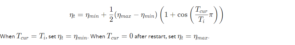
Cosine Annhealing Learning Rate
It sets the learning rate of each parameter group using a cosine annealing schedule, where ηmax is set to the initial lr and Tcur is the number of epochs since the last restart in SGDR
When last_epoch=-1, sets initial lr as lr. Notice that because the schedule is defined recursively, the learning rate can be simultaneously modified outside this scheduler by other operators. If the learning rate is set solely by this scheduler, the learning rate at each step becomes

This has been proposed in SGDR: Stochastic Gradient Descent with Warm Restarts. Note that this only implements the cosine annealing part of SGDR, and not the restarts.
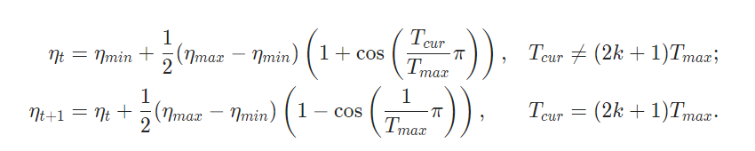
Cosine Annealing Warm Restarts
It sets the learning rate of each parameter group using a cosine annealing schedule, where ηmax is set to the initial lr, Tcur is the number of epochs since the last restart and Ti is the number of epochs between two warm restarts in SGDR
It has been proposed in SGDR: Stochastic Gradient Descent with Warm Restarts.
def fetch_scheduler(optimizer):

    if CONFIG['scheduler'] == 'CosineAnnealingLR':
        scheduler = lr_scheduler.CosineAnnealingLR(
            optimizer,
            T_max=CONFIG['T_max'],
            eta_min=CONFIG['min_lr']
        )

    elif CONFIG['scheduler'] == 'CosineAnnealingWarmRestarts':
        scheduler = lr_scheduler.CosineAnnealingWarmRestarts(
            optimizer,
            T_0=CONFIG['T_0'],
            eta_min=CONFIG['min_lr']
        )

    elif CONFIG['scheduler'] == None:
        return None

    return scheduler
wandb_logger is created to log specified data (in this case, the losses) to Weights and Biases.
# W&B Logger
wandb_logger = WandbLogger(
    project='jigsaw-lightning',
    job_type='train',
    anonymous='allow',
    config=CONFIG
)
Dataset
The dataset used has two important columns namely less_toxic and more_toxic and as the name suggests one contains a less toxic comment and another contains the more toxic comment. It has another column namely worker which is the id of the annotator.
Now that we have our configuration and utilities prepared, we can move towards preparing the dataset class. While working in PyTorch/PyTorch Lightning you need to define a dataset class that extends the Dataset module imported earlier.
The dataset module has three functions -
__init__: The__init__function is run once when instantiating the Dataset object.__len__: The__len__function returns the number of samples in our dataset.- The
__getitem__function loads and returns a sample from the dataset at the given indexindex. Based on the index, it identifies the data location on disk, encodes the data, and sets thetarget = 1.Finally it returnstensorsof theids, mask, target.Remember that we are using therobertamodel here which does not havetoken_type_ids.
Now you might have a question that why and how did we set the target = 1 in the below block of code! Wait a bit and you will have your answer.
class JigsawDataset(Dataset):
    def __init__(self, df, tokenizer, max_length):
        self.df = df
        self.max_len = max_length
        self.tokenizer = tokenizer
        self.more_toxic = df['more_toxic'].values
        self.less_toxic = df['less_toxic'].values

    def __len__(self):
        return len(self.df)

    def __getitem__(self, index):
        more_toxic = self.more_toxic[index]
        less_toxic = self.less_toxic[index]
        inputs_more_toxic = self.tokenizer.encode_plus(
                                more_toxic,
                                truncation=True,
                                add_special_tokens=True,
                                max_length=self.max_len,
                                padding='max_length'
                            )
        inputs_less_toxic = self.tokenizer.encode_plus(
                                less_toxic,
                                truncation=True,
                                add_special_tokens=True,
                                max_length=self.max_len,
                                padding='max_length'
                            )
        target = 1

        more_toxic_ids = inputs_more_toxic['input_ids']
        more_toxic_mask = inputs_more_toxic['attention_mask']

        less_toxic_ids = inputs_less_toxic['input_ids']
        less_toxic_mask = inputs_less_toxic['attention_mask']

        return {
            'more_toxic_ids': torch.tensor(more_toxic_ids, dtype=torch.long),
            'more_toxic_mask': torch.tensor(more_toxic_mask, dtype=torch.long),
            'less_toxic_ids': torch.tensor(less_toxic_ids, dtype=torch.long),
            'less_toxic_mask': torch.tensor(less_toxic_mask, dtype=torch.long),
            'target': torch.tensor(target, dtype=torch.long)
        }
DataModule
Pytorch Lightning provides an additional datamodule which is a shareable, reusable class that encapsulates all the steps needed to process data.
It is simply a collection of a train_dataloader(s), val_dataloader(s), test_dataloader(s) and predict_dataloader(s) along with the matching transforms and data processing/downloads steps required.
A data module encapsulates the five steps involved in data processing in PyTorch:
- Download / tokenize / process.
- Clean and (maybe) save to disk.
- Load inside Dataset.
- Apply transforms (rotate, tokenize, etc.)
- Wrap inside a DataLoader.
Now you may have another question. Is it necessary to use the DataModule?
The answer is No. You can write all the code separately as well, but the DataModule helps to encapsulate all of it in one place making your code more readable and sharable.
class JigsawDataModule(pl.LightningDataModule):

  def __init__(self, df_train, df_valid):
    super().__init__()
    self.df_train = df_train
    self.df_valid = df_valid

  def setup(self, stage=None):

    self.train_dataset = JigsawDataset(
        self.df_train,
        tokenizer = CONFIG['tokenizer'],
        max_length=CONFIG['max_length']
    )

    self.valid_dataset = JigsawDataset(
        self.df_valid,
        tokenizer=CONFIG['tokenizer'],
        max_length=CONFIG['max_length']
    )

  def train_dataloader(self):
    return DataLoader(
      self.train_dataset,
      batch_size=CONFIG['train_batch_size'],
      num_workers=CONFIG["num_workers"],
      shuffle=True,
      pin_memory=True,
      drop_last=True
    )

  def val_dataloader(self):
    return DataLoader(
      self.valid_dataset,
      batch_size=CONFIG['valid_batch_size'],
      num_workers=CONFIG["num_workers"],
      shuffle=False,
      pin_memory=True
    )
Model
And finally, we have reached the most interesting part, Modeling!
But before we move into the world of Transformers let's first define the Loss Function that we will be using.
Margin Ranking Loss
Since no Target variable is present in the dataset (remember we explicitly specified Target = 1 in the dataset class), we use the Margin Ranking Loss
It creates a criterion that measures the loss given inputs x1, x2, two 1D mini-batch Tensors, and a label 1D mini-batch tensor y (containing 1 or -1).
If y = 1, then it assumed the first input should be ranked higher (should have a larger value) than the second input, and vice-versa for y = -1.
For the same reason, we set Target = 1 earlier.
The loss function for each pair of samples in the mini-batch is:
loss(x1, x2, y) = max(0, -y * (x1 - x2) + margin)
Refer to docs to understand all the parameters.
RoBERTa
RoBERTa stands for Robustly Optimized Bidirectional Encoder Representations from Transformers.
RoBERTa is an extension of BERT with changes to the pretraining procedure. The modifications include:
- Training the model longer, with bigger batches, over more data
- Removing the next sentence prediction objective
- Training on longer sequences
- Dynamically changing the masking pattern applied to the training data. The authors also collect a large new dataset of comparable size to other privately used datasets, to better control for training set size effects.
It was proposed in 2019 by Yinhan Liu Et. al. in RoBERTa: A Robustly Optimized BERT Pretraining Approach
class JigsawModel(pl.LightningModule):

    def __init__(self, model_name):
        super(JigsawModel, self).__init__()
        self.model = AutoModel.from_pretrained(model_name)
        self.drop = nn.Dropout(p=0.2)
        self.fc = nn.Linear(768, CONFIG['num_classes'])

    def forward(self, ids, mask):
        out = self.model(input_ids=ids,attention_mask=mask,
                         output_hidden_states=False)
        out = self.drop(out[1])
        outputs = self.fc(out)

        return outputs

    def training_step(self, batch, batch_idx):
        more_toxic_ids = batch['more_toxic_ids']
        more_toxic_mask = batch['more_toxic_mask']
        less_toxic_ids = batch['less_toxic_ids']
        less_toxic_mask = batch['less_toxic_mask']
        targets = batch['target']

        more_toxic_outputs = self(more_toxic_ids, more_toxic_mask)
        less_toxic_outputs = self(less_toxic_ids, less_toxic_mask)

        loss = self.criterion(more_toxic_outputs, less_toxic_outputs, targets)

        self.log("train_loss", loss, prog_bar=True, logger=True)

        return {"loss": loss}

    def validation_step(self, batch, batch_idx):
        more_toxic_ids = batch['more_toxic_ids']
        more_toxic_mask = batch['more_toxic_mask']
        less_toxic_ids = batch['less_toxic_ids']
        less_toxic_mask = batch['less_toxic_mask']
        targets = batch['target']

        more_toxic_outputs = self(more_toxic_ids, more_toxic_mask)
        less_toxic_outputs = self(less_toxic_ids, less_toxic_mask)

        loss = self.criterion(more_toxic_outputs, less_toxic_outputs, targets)

        self.log("val_loss", loss, prog_bar=True, logger=True)

        return {'val_loss': loss}

    def configure_optimizers(self):

        optimizer = AdamW(self.parameters(), lr=CONFIG['learning_rate'], weight_decay=CONFIG['weight_decay'])
        scheduler = fetch_scheduler(optimizer)

        return dict(
            optimizer = optimizer,
            lr_scheduler = scheduler
        )

    def criterion(self, outputs1, outputs2, targets):
        return nn.MarginRankingLoss(margin=CONFIG['margin'])(outputs1, outputs2, targets)
The above model definition is simple. If you are already familiar with PyTorch, what happens above is instead of writing loops separately, you put the code in separate functions and Lightning takes care of the rest.
Understanding Mixed Precision
We use a method known as Mixed Precision to optimize our model.
Introduction
There are numerous benefits to using numerical formats with lower precision than 32-bit floating-point:
- They require less memory, enabling the training and deployment of larger neural networks.
- They require less memory bandwidth, thereby speeding up data transfer operations.
- Math operations run much faster in reduced precision, especially on GPUs with Tensor Core support for that precision.
Mixed precision training achieves all these benefits while ensuring that no task-specific accuracy is lost compared to full precision training. It does so by identifying the steps that require full precision and using a 32-bit floating-point for only those steps while using a 16-bit floating-point everywhere else.
Mixed Precision Training
Mixed precision training offers significant computational speedup by performing operations in the half-precision format while storing minimal information in single-precision to retain as much information as possible in critical parts of the network.
Since the introduction of Tensor Cores in the Volta and Turing architectures, significant training speedups are experienced by switching to mixed-precision -- up to 3x overall speedup on the most arithmetically intense model architectures.
Using mixed-precision training requires two steps:
- Porting the model to use the FP16 data type wherever appropriate.
- Adding loss scaling to preserve small gradient values.
The ability to train deep learning networks with lower precision was introduced in the Pascal architecture and first supported in CUDA® 8 in the NVIDIA Deep Learning SDK.
Mixed precision is the combined use of different numerical precisions in a computational method.
Half precision (also known as FP16) data compared to higher precision FP32 vs FP64 reduces memory usage of the neural network, allowing training and deployment of larger networks, and FP16 data transfers take less time than FP32 or FP64 transfers.
Single precision (also known as 32-bit) is a common floating-point format (float in C-derived programming languages), and 64-bit, known as double-precision (double).
Deep Neural Networks (DNNs) have led to breakthroughs in several areas, including image processing and understanding, language modeling, language translation, speech processing, game playing, and many others. DNN complexity has been increasing to achieve these results, which in turn has increased the computational resources required to train these networks.
One way to lower the required resources is to use lower-precision arithmetic, which has the following benefits.
Decrease the required amount of memory: Half-precision floating-point format (FP16) uses 16 bits, compared to 32 bits for single-precision (FP32). Lowering the required memory enables training of larger models or training with larger mini-batches.
Shorten the training or inference time: Execution time can be sensitive to memory or arithmetic bandwidth. Half-precision halves the number of bytes accessed, thus reducing the time spent in memory-limited layers. NVIDIA GPUs offer up to 8x more half-precision arithmetic throughput when compared to single-precision, thus speeding up math-limited layers.
Read NVIDIA Docs for additional examples.
Training
With the data, model and hardware prepared we are now ready to train the model.
We use 5 Fold Training as a Cross-Validation Strategy here.
if __name__ == "__main__":
    for fold in range(0, CONFIG['n_fold']):
        print(f"{y_}====== Fold: {fold} ======{sr_}")

                # Load Dataset
        df = pd.read_csv(CONFIG['train_file_path'])

                # Set the Training and Validation Data for current fold
                df_train = df[df.kfold != fold].reset_index(drop=True)
        df_valid = df[df.kfold == fold].reset_index(drop=True)

                # Declare Model Checkpoint
        checkpoint_callback = ModelCheckpoint(
          dirpath=CONFIG["checkpoint_directory_path"],
          filename= f"fold_{fold}_roberta-base",
          save_top_k=1,
          verbose=True,
          monitor="val_loss",
          mode="min"
        )

                # Early Stopping based on Validation Loss
        early_stopping_callback = EarlyStopping(monitor='val_loss', patience=2)

                # Initialise the Trainer
        trainer = pl.Trainer(
          logger=wandb_logger,
          callbacks=[checkpoint_callback, early_stopping_callback],
          max_epochs=CONFIG['epochs'],
          gpus=-1,
          progress_bar_refresh_rate=30,
          precision=16,                # Activate fp16 Training
#accelerator = 'dp'         # Uncomment for Multi-GPU Training
        )

        data_module = JigsawDataModule(df_train, df_valid)
        model = JigsawModel(CONFIG['model_name'])

        trainer.fit(model, data_module)
The code is also compatible with a multi-GPU training setup. If you have more than one GPU in one machine set the accelerator = dp
You can view the Weights and Biases Run Page here.
Conclusion
Thus, you have successfully created a Deep Learning Model to Rank relative ratings of toxicity between comments. Here I had used roberta-base but you could experiment with larger models like roberta-large.
How can you improve your model further?
You can try out different techniques such as:
- Train on additional external Data
- Gradient Accumulation
- Gradient Clipping
- Grouped Layerwise Learning Rate Decay
- Utilizing Intermediate Transformer Representations
- Layer Initialization
- Model Ensembling
Code Notebook
The Code present in the article is available in this notebook on Kaggle. Give it a try and try to make suggested changes!
Reach Out to Me
If you have any doubts about the blog or would like to have a talk you can reach out to me on LinkedIn or Twitter, I would be happy to help!